In spite of both theorecital and empirical evidence to the contrary, it is often assumed that grades are or should be normally distributed. This has important implications for how we understand and analyze these data-points within learning analytics. In this blog posts I will take a look at some of the theoretical assumtions surrounding the normal distribution and how it applies to grading data, and offer some proposals on what to do when these assumptions are not met.

The Theory

The normal distribution (AKA Gaussian or LaPlace-Gauss distribution) is defined by two parameters its mean (\(\mu\)) and variance (\(\sigma^2\)). The normal distribution is further a continuous distribution and its limits are -\(\infty\) to \(\infty\).

We can already see that there are some problems with this relating to grade data. Firstly, grades are not given on a continuous scale. Letter-grades are typically gives as say A+, A and A- etcetera, and even in locations where number grades are common, one rarely sees decimal expansions beyond a tick of one half-grade, e.g. 9.5/10 and so on. So grades are given on a discrete scale of some sort. Secondly, grades are limited to a maximum grade and minimum grade, it is clearly not possible to receive a negative grade.

Why Does It Matter?

A lot of techniques used for modeling data and conducting inferential analyses are based on the assumtion that the data under analysis follow a normal distributions. Well knows methods such as linear regression, the z-test and Student’s T-Test all rely on this assumption.

A Practical Example

The data below are final grades from two different sections (Group A and Group B) of the same course. The researcher has experimented with different courseware for each of the section and wants to know if the courseware made a difference. The grades are assigned on scale from zero to ten. Let’s take a look at how these data can be analyzed.

Group.A <- c(7.5, 10, 7.5, 8, 10, 4, 4, 6, 8, 4, 4, 8, 9, 4, 5, 6, 5, 9, 4, 5, 4, 7, 5, 4, 4, 4, 9, 6, 4)

Group.B <- c(5, 5.5, 9, 9, 9, 7, 4, 6, 6, 6, 8.5, 8, 10, 5.5, 10, 2, 9, 5, 9, 7.5, 9, 9, 10, 10, 7, 4, 7, 4, 5, 6, 6, 10, 5, 9, 4)

The Fast and Furious Approach

mean(Group.A)

## [1] 6.034483

mean(Group.B)

## [1] 7.028571

We see that there is a difference of about one point between the two groups, i.e. about 10%. Now we would like to know if the difference is statistically significant, i.e. if we can reasonably conclude that the difference is not due to just random variation. The go-to technique for this case is Student’s t-test.

t.test(Group.A, Group.B)

## 
##  Welch Two Sample t-test
## 
## data:  Group.A and Group.B
## t = -1.8346, df = 60.781, p-value = 0.07145
## alternative hypothesis: true difference in means is not equal to 0
## 95 percent confidence interval:
##  -2.07765141  0.08947407
## sample estimates:
## mean of x mean of y 
##  6.034483  7.028571

We see that while there is a difference in the mean between the two groups it does not reach the level of statistical significance, typically defined as an alpha-level of .05.

Tough luck! We’ll try again next semester…

The Rigorous Approach

Always visualize! It is typically a good idea to visualize the data we’re analyzing to get a sense for its structure and shape. This will also, incidentally, aid in the detection of outliers, data-entry mistakes and other problems in the data that we would want to deal with before proceeding with the analysis. Here we plot the density of each of the groups using R and ggplot:

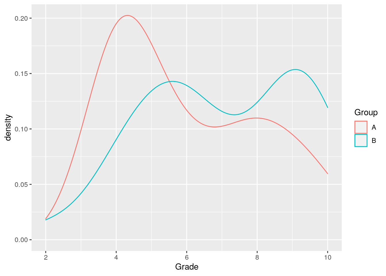
By looking at this plot we may start to suspect that our samples are not normally distributed. There are some statistical tests that can be used to formally test this. One of them is the Shapiro-Wilk Test.

This techique tests the null-hypothesis of a normal distribution and calculates a corresponding p-level. It is often recommended to use an alpha-level of .1 when applying this test, to err on the side of caution. It is convenienty available in R:

shapiro.test(Group.A)

## 
##  Shapiro-Wilk normality test
## 
## data:  Group.A
## W = 0.8444, p-value = 0.0005847

shapiro.test(Group.B)

## 
##  Shapiro-Wilk normality test
## 
## data:  Group.B
## W = 0.92425, p-value = 0.01894

We see that neither of the two groups conforms to a normal distribution, so the using a t-test is actually not appropriate. Luckily we have a non-parametric alternative, the Wilcox Rank Sum Test. This test is also conveniently available in R.

wilcox.test(Group.A, Group.B)

## 
##  Wilcoxon rank sum test with continuity correction
## 
## data:  Group.A and Group.B
## W = 362.5, p-value = 0.04859
## alternative hypothesis: true location shift is not equal to 0

We have a p-value below our selected alpha-level of .05, and can therefore reject the null-hypothesis of no real difference between the two groups.

Conclusion

Not testing for the assumption of normality can lead to undesired consequences for inferential analysis. In the example above, we see that the vanilla t-test fails to reject our null-hypothesis, however, its non-parametric counterpart succeeds. By adopting a somewhat more rigorous approach we were able to select the correct statistical test and uncover patterns in our data that the parametric test could not.

Not Normal!